Housing Regression

This dataset is composed of over 20,000 rows and 9 columns.

Notebook goals:

Complete regression analysis with train-test split and two models for comparison
Data investigation of summary statistics and visualizations
Metric evaluation and performance visualization

Imports

# import os
# import numpy as np
import pandas as pd
# import seaborn as sns
# import matplotlib.pyplot as plt
from skimpy import skim
import plotly.express as px

from sklearn.datasets import fetch_california_housing
from sklearn.model_selection import train_test_split
from sklearn.linear_model import LinearRegression
from sklearn.ensemble import RandomForestRegressor
from sklearn.metrics import (
    mean_squared_error,
    explained_variance_score
)

Data

Get the Data

Import the data from sklearn
Transfer data into pandas DataFrame
Basic data overview

Note: Data is returned as a bunch object, similar to a dictionary. We’ll convert it to a pandas df.

# Load data
data = fetch_california_housing()

type(data)

sklearn.utils._bunch.Bunch

data.keys()

dict_keys(['data', 'target', 'frame', 'target_names', 'feature_names', 'DESCR'])

# Convert data to pandas dataframe
df = pd.DataFrame(data=data['data'], columns=data['feature_names'])

df.head()

	MedInc	HouseAge	AveRooms	AveBedrms	Population	AveOccup	Latitude	Longitude
0	8.3252	41.0	6.984127	1.023810	322.0	2.555556	37.88	-122.23
1	8.3014	21.0	6.238137	0.971880	2401.0	2.109842	37.86	-122.22
2	7.2574	52.0	8.288136	1.073446	496.0	2.802260	37.85	-122.24
3	5.6431	52.0	5.817352	1.073059	558.0	2.547945	37.85	-122.25
4	3.8462	52.0	6.281853	1.081081	565.0	2.181467	37.85	-122.25

df.shape

(20640, 8)

Add target to df

df["target"] = data['target']

df.head()

	MedInc	HouseAge	AveRooms	AveBedrms	Population	AveOccup	Latitude	Longitude	target
0	8.3252	41.0	6.984127	1.023810	322.0	2.555556	37.88	-122.23	4.526
1	8.3014	21.0	6.238137	0.971880	2401.0	2.109842	37.86	-122.22	3.585
2	7.2574	52.0	8.288136	1.073446	496.0	2.802260	37.85	-122.24	3.521
3	5.6431	52.0	5.817352	1.073059	558.0	2.547945	37.85	-122.25	3.413
4	3.8462	52.0	6.281853	1.081081	565.0	2.181467	37.85	-122.25	3.422

# NOTE: 1 additional column
df.shape

(20640, 9)

Explore Dataset

df.info()

<class 'pandas.core.frame.DataFrame'>
RangeIndex: 20640 entries, 0 to 20639
Data columns (total 9 columns):
 #   Column      Non-Null Count  Dtype  
---  ------      --------------  -----  
 0   MedInc      20640 non-null  float64
 1   HouseAge    20640 non-null  float64
 2   AveRooms    20640 non-null  float64
 3   AveBedrms   20640 non-null  float64
 4   Population  20640 non-null  float64
 5   AveOccup    20640 non-null  float64
 6   Latitude    20640 non-null  float64
 7   Longitude   20640 non-null  float64
 8   target      20640 non-null  float64
dtypes: float64(9)
memory usage: 1.4 MB

skim(df)

╭──────────────────────────────────────────────── skimpy summary ─────────────────────────────────────────────────╮
│          Data Summary                Data Types                                                                 │
│ ┏━━━━━━━━━━━━━━━━━━━┳━━━━━━━━┓ ┏━━━━━━━━━━━━━┳━━━━━━━┓                                                          │
│ ┃ Dataframe         ┃ Values ┃ ┃ Column Type ┃ Count ┃                                                          │
│ ┡━━━━━━━━━━━━━━━━━━━╇━━━━━━━━┩ ┡━━━━━━━━━━━━━╇━━━━━━━┩                                                          │
│ │ Number of rows    │ 20640  │ │ float64     │ 9     │                                                          │
│ │ Number of columns │ 9      │ └─────────────┴───────┘                                                          │
│ └───────────────────┴────────┘                                                                                  │
│                                                     number                                                      │
│ ┏━━━━━━━━━━━━━━┳━━━━━┳━━━━━━━┳━━━━━━━━━━┳━━━━━━━━━━┳━━━━━━━━━┳━━━━━━━━━┳━━━━━━━━━┳━━━━━━━━┳━━━━━━━━━┳━━━━━━━━┓  │
│ ┃ column       ┃ NA  ┃ NA %  ┃ mean     ┃ sd       ┃ p0      ┃ p25     ┃ p50     ┃ p75    ┃ p100    ┃ hist   ┃  │
│ ┡━━━━━━━━━━━━━━╇━━━━━╇━━━━━━━╇━━━━━━━━━━╇━━━━━━━━━━╇━━━━━━━━━╇━━━━━━━━━╇━━━━━━━━━╇━━━━━━━━╇━━━━━━━━━╇━━━━━━━━┩  │
│ │ MedInc       │   0 │     0 │    3.871 │      1.9 │  0.4999 │   2.563 │   3.535 │  4.743 │      15 │  ▆█▂   │  │
│ │ HouseAge     │   0 │     0 │    28.64 │    12.59 │       1 │      18 │      29 │     37 │      52 │ ▂▆███▅ │  │
│ │ AveRooms     │   0 │     0 │    5.429 │    2.474 │  0.8462 │   4.441 │   5.229 │  6.052 │   141.9 │   █    │  │
│ │ AveBedrms    │   0 │     0 │    1.097 │   0.4739 │  0.3333 │   1.006 │   1.049 │    1.1 │   34.07 │   █    │  │
│ │ Population   │   0 │     0 │     1425 │     1132 │       3 │     787 │    1166 │   1725 │   35680 │   █    │  │
│ │ AveOccup     │   0 │     0 │    3.071 │    10.39 │  0.6923 │    2.43 │   2.818 │  3.282 │    1243 │   █    │  │
│ │ Latitude     │   0 │     0 │    35.63 │    2.136 │   32.54 │   33.93 │   34.26 │  37.71 │   41.95 │ █▃▁▆▁  │  │
│ │ Longitude    │   0 │     0 │   -119.6 │    2.004 │  -124.3 │  -121.8 │  -118.5 │   -118 │  -114.3 │ ▁▆▂█▃  │  │
│ │ target       │   0 │     0 │    2.069 │    1.154 │    0.15 │   1.196 │   1.797 │  2.647 │       5 │ ▄█▆▃▂▂ │  │
│ └──────────────┴─────┴───────┴──────────┴──────────┴─────────┴─────────┴─────────┴────────┴─────────┴────────┘  │
╰────────────────────────────────────────────────────── End ──────────────────────────────────────────────────────╯

Train-Test Split

Splitting data before EDA can be helpful to avoid data leakage or incorrect assumptions about what the data shows.

EDA and training will use only the train data. Test data will be used for evaluation only.

Note: Splitting is normally done with X (features) and y (target) separated to avoid data leakage. Here, we will training and test data and split X, y before model training.

X_train, X_test, y_train, y_test = train_test_split(X, y, test_size=0.33, random_state=42)

train_df, test_df = train_test_split(df, test_size=0.33, random_state=42)

EDA

print(f'Shape of original data: {df.shape}')
print(f'Shape of training data: {train_df.shape}')
print(f'Shape of training data: {test_df.shape}')

Shape of original data: (20640, 9)
Shape of training data: (13828, 9)
Shape of training data: (6812, 9)

print(f'Percent of data in training: {len(train_df)/len(df):.0%}')
print(f'Percent of data in test: {len(test_df)/len(df):.0%}')

Percent of data in training: 67%
Percent of data in test: 33%

Focus on Train for EDA

It is best not to peek at test data. It can lead to unsupported assumptions.

skim(train_df)

╭──────────────────────────────────────────────── skimpy summary ─────────────────────────────────────────────────╮
│          Data Summary                Data Types                                                                 │
│ ┏━━━━━━━━━━━━━━━━━━━┳━━━━━━━━┓ ┏━━━━━━━━━━━━━┳━━━━━━━┓                                                          │
│ ┃ Dataframe         ┃ Values ┃ ┃ Column Type ┃ Count ┃                                                          │
│ ┡━━━━━━━━━━━━━━━━━━━╇━━━━━━━━┩ ┡━━━━━━━━━━━━━╇━━━━━━━┩                                                          │
│ │ Number of rows    │ 13828  │ │ float64     │ 9     │                                                          │
│ │ Number of columns │ 9      │ └─────────────┴───────┘                                                          │
│ └───────────────────┴────────┘                                                                                  │
│                                                     number                                                      │
│ ┏━━━━━━━━━━━━━━┳━━━━━┳━━━━━━━┳━━━━━━━━━━┳━━━━━━━━━━┳━━━━━━━━━┳━━━━━━━━━┳━━━━━━━━━┳━━━━━━━━┳━━━━━━━━━┳━━━━━━━━┓  │
│ ┃ column       ┃ NA  ┃ NA %  ┃ mean     ┃ sd       ┃ p0      ┃ p25     ┃ p50     ┃ p75    ┃ p100    ┃ hist   ┃  │
│ ┡━━━━━━━━━━━━━━╇━━━━━╇━━━━━━━╇━━━━━━━━━━╇━━━━━━━━━━╇━━━━━━━━━╇━━━━━━━━━╇━━━━━━━━━╇━━━━━━━━╇━━━━━━━━━╇━━━━━━━━┩  │
│ │ MedInc       │   0 │     0 │    3.877 │    1.903 │  0.4999 │   2.569 │   3.539 │  4.757 │      15 │  ▅█▂   │  │
│ │ HouseAge     │   0 │     0 │    28.56 │     12.6 │       1 │      18 │      29 │     37 │      52 │ ▂▆███▅ │  │
│ │ AveRooms     │   0 │     0 │    5.437 │    2.449 │  0.8889 │    4.46 │   5.232 │  6.059 │   141.9 │   █    │  │
│ │ AveBedrms    │   0 │     0 │    1.098 │   0.4457 │  0.3333 │   1.007 │    1.05 │    1.1 │   25.64 │   █    │  │
│ │ Population   │   0 │     0 │     1431 │     1146 │       3 │     793 │    1170 │   1729 │   35680 │   █    │  │
│ │ AveOccup     │   0 │     0 │    3.129 │    12.65 │  0.6923 │   2.432 │    2.82 │  3.282 │    1243 │   █    │  │
│ │ Latitude     │   0 │     0 │    35.65 │    2.134 │   32.55 │   33.94 │   34.27 │  37.72 │   41.95 │ █▃▁▆▁  │  │
│ │ Longitude    │   0 │     0 │   -119.6 │    2.005 │  -124.3 │  -121.8 │  -118.5 │   -118 │  -114.3 │ ▁▆▂█▃  │  │
│ │ target       │   0 │     0 │    2.067 │    1.154 │    0.15 │   1.194 │   1.792 │   2.64 │       5 │ ▄█▆▃▂▂ │  │
│ └──────────────┴─────┴───────┴──────────┴──────────┴─────────┴─────────┴─────────┴────────┴─────────┴────────┘  │
╰────────────────────────────────────────────────────── End ──────────────────────────────────────────────────────╯

All Features and Target are Numeric

A loop can help iterate over the columns and produce visualizations.

col_list = train_df.columns.to_list()

col_list

['MedInc',
 'HouseAge',
 'AveRooms',
 'AveBedrms',
 'Population',
 'AveOccup',
 'Latitude',
 'Longitude',
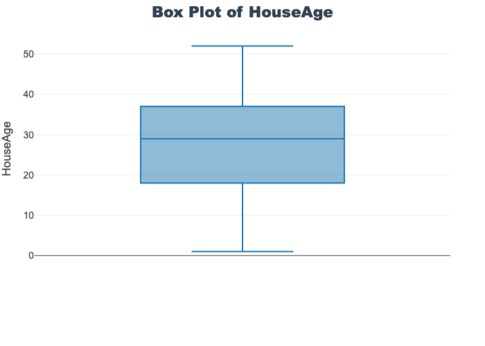
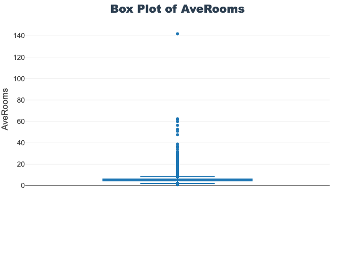
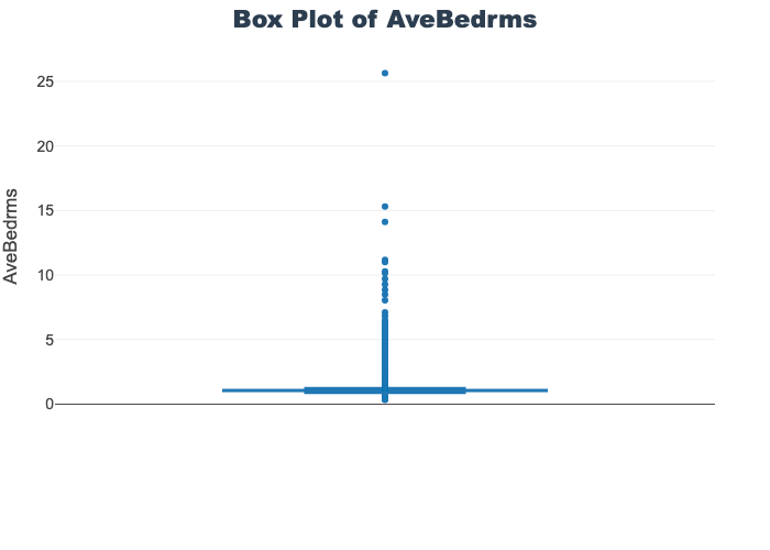
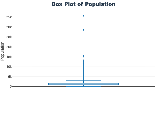
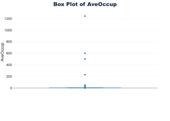
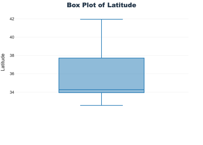
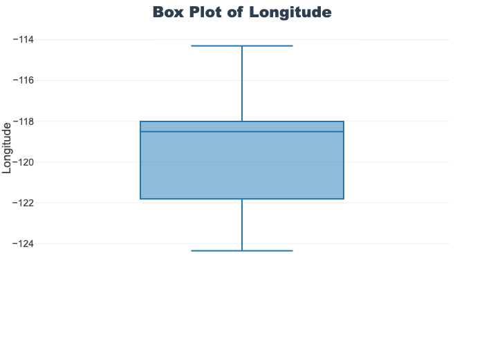
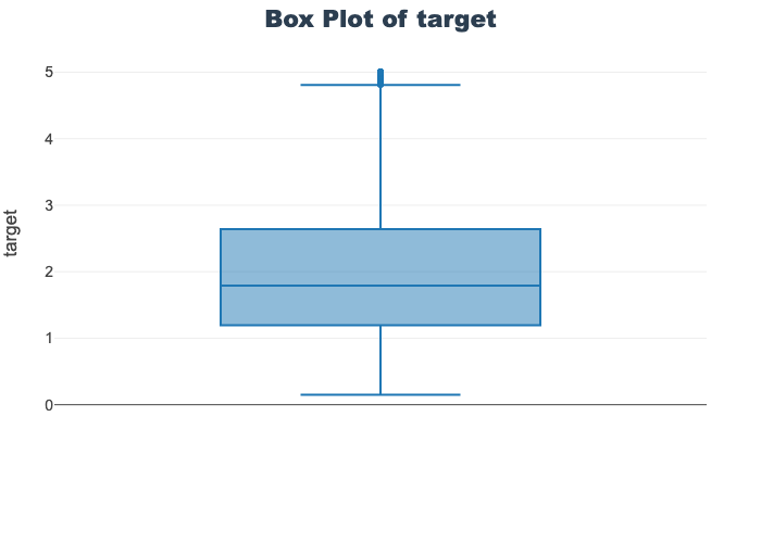
 'target']

for col in col_list:
    fig = px.box(train_df, y=col, title=f'Box Plot of {col}')
    fig.show()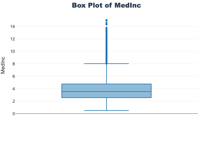

# px.box(sepal_df, x="species", y="value", 
#              facet_col="variable", title="Sepal Features by Species",
#              color="species")

train_df.columns

Index(['MedInc', 'HouseAge', 'AveRooms', 'AveBedrms', 'Population', 'AveOccup',
       'Latitude', 'Longitude', 'target'],
      dtype='object')

Model Training

# Instantiate model, fit model, save model
lr = LinearRegression()
lr.fit(X_train, y_train)

---------------------------------------------------------------------------
NameError                                 Traceback (most recent call last)
Cell In[21], line 3
      1 # Instantiate model, fit model, save model
      2 lr = LinearRegression()
----> 3 lr.fit(X_train, y_train)

NameError: name 'X_train' is not defined

# Instantiate model, fit model, save model
rf = RandomForestRegressor()
rf.fit(X_train, y_train)

# Predict on train with both models
# NOTE: test metrics are more insightful
lr_train_preds = lr.predict(X_train)
rf_train_preds = rf.predict(X_train)

# Calculate mean squared error for both models
lr_mse = mean_squared_error(y_train, lr_train_preds)
rf_mse = mean_squared_error(y_train, rf_train_preds)

# Print calculations
print(f"The MSE for the linear regression models is : {lr_mse: .2f}")
print(f"The MSE for the random forest regression models is : {rf_mse: .2f}")

# Plot both predictions
plt.figure(figsize=(10,10))
plt.scatter(y_train, lr_train_preds, c='crimson', label='Linear Regression')
plt.scatter(y_train, rf_train_preds, c='gold', label='RF Regression')

plt.xlabel('True Values', fontsize=15)
plt.ylabel('Predictions', fontsize=15)
plt.title('Training Error', fontsize=15)

plt.legend()
plt.tight_layout()
plt.show()

Evaluate Models Notebook

# linear regression predict
lr_preds = lr.predict(X_test)
lr_preds

# random forest regression predict
rf_preds = rf.predict(X_test)
rf_preds

# Calculate explained variance for both models
lr_evs = explained_variance_score(y_test, lr_preds)
rf_evs = explained_variance_score(y_test, rf_preds)

# Display explained variance scores
print(f'The explained variance score for the linear regression models is: {lr_evs: .2f}')
print(f'The explained variance score for the random forest regression models is: {rf_evs: .2f}')

# Calculate mean squared error (MSE)
lr_mse = mean_squared_error(y_test, lr_preds)
rf_mse = mean_squared_error(y_test, rf_preds)

# Display MSE
print(f"The MSE for the linear regression models is : {lr_mse: .2f}")
print(f"The MSE for the random forest regression models is : {rf_mse: .2f}")

# create y_df with real and predicted values
y_df=pd.DataFrame({'y_true': y_test, 'lr_preds': lr_preds, 'rf_preds': rf_preds})

# Check df
y_df.head()

# Get correlation across real, lr, and rf values
y_df.corr()

# Seaborn pair plot on y data
sns.pairplot(y_df)

# Plot results
plt.figure(figsize=(10,10))
plt.scatter(y_test.target, lr_preds, c='crimson', label='Linear Regression')
plt.scatter(y_test.target, rf_preds, c='gold', label='RF Regression')

plt.xlabel('True Values', fontsize=15)
plt.ylabel('Predictions', fontsize=15)
plt.title('Test Error', fontsize=15)

plt.legend()
plt.tight_layout()
plt.show()